During lifecycle development of a biological assay (bioassay), identifying and reducing sources of variability might be required to improve method performance. Here I recommend some statistical and graphical approaches (consistent with USP <1033>) for practitioners to identify variation from experimental results (1).
Sources of Variation in a Bioassay
To correctly identify sources of variation in a bioassay, analysts must consider how that bioassay is to be executed. In particular, the experience and technical expertise of each analyst expected to execute the bioassay should be taken into account. If the dataset used in a variability study contains results predominantly from highly trained and experienced analysts, the estimate of precision can be disingenuously better (smaller variation) than with a more diverse level of technical aptitude across the analyst population. Conversely, if analyzed results emanate from inexperienced analysts, an estimate of precision can be worse (larger variation) than expected. Other frequently considered sources of variation in a bioassay can include day-to-day variation, critical reagent lot variation, and inter- and intra-assay (also known as repeatability) variation. Once analysts establish a dataset that reasonably can be expected to identify key sources of variation, the following assessments would be meaningful.
Overview of Variance Components
As recommended in USP <1033>, sources of variation can be estimated using variance component analysis (1). To obtain point estimates of the true variance component value, results from a variability study typically are entered into a statistical software package for ease of calculation. If the factor in a bioassay study is considered a random effect (if it represents an expected source of random method variation), then the point estimate of each variance component and the associated percentage of total variation can be considered.
With bioassay data, analysts recommend the use of a logarithm base e data transformation on relative-potency results before performing calculations. This transformation reduces the impact of variance heterogeneity with increasing potency (2) and allows for a direct comparison of results separately across nominal levels, as shown in Table 6 of USP <1033>.
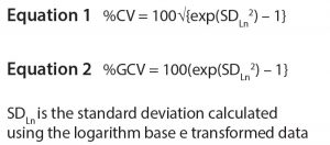
The percentage of variation attributable to each assessed source is a useful byproduct of the variance component analysis. Numeric results for the variance component estimates (calculated using the logarithm-transformed data) can be difficult to interpret from a practical standpoint. For example, output from a statistical software package would list each component (and variance component estimate) such as a value of 0.0051. Using the variance component estimate is preferred to obtain a more familiar statistic such as the percentage coefficient of variation (%CV) or the percentage geometric coefficient of variation (%GCV). Those are calculated as shown in Table A-1 of USP <1033> and herein as Equations 1 and 2, respectively. For example, with a variance component estimate of 0.0051, %CV is 100*√{exp(0.0051) – 1} ≈ 7.2%, and %GCV is 100*(exp(√0.0051) – 1) ≈ 7.4%.
As noted in USP <1033>, %GCV is a measure relevant to the logarithm-transformed data, whereas %CV is relevant to the original units of the metric. If the estimate of variation is relatively low (e.g., %CV < 20%), there is a minimal difference in the estimates of %GCV and %CV from a practical perspective. Correspondingly, %CV typically is used more widely by practitioners who have developed well-behaved bioassays.
Illustration of Variability Studies
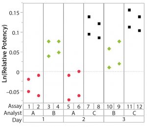
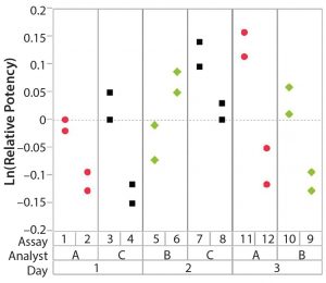
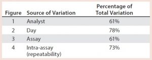
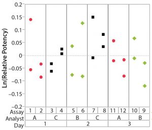
After having collected a library of data from executed bioassays, analysts most readily can understand the variance component estimates and the corresponding percentage of variation by using a graphical representation. Examples are not provided in USP <1033>, so they are addressed here as recommended practice. Table 1 indicates the highest component of variation in each of Figures 1–4. The simulated results are from a design based on the work of three analysts over the course of three days, with different simulated data used for each figure. Two assays were performed by each analyst on a given day, and each combination of analyst/day is captured in the variability study.
The type of statistical and graphical analyses of experimental data shown here are recommended for practitioners wanting to identify and address sources of variation when performing a bioassay. The information provided by those results can provide valuable insights and enables more appropriately focused efforts to reduce bioassay variability.
References
1 <1033> Biological Assay Validation. USP 40-NF 35. The United States Pharmacopeial Convention: Rockville, MD, 2017.
2 <1032> Design and Development of Biological Assays, Section 4.3. USP 40-NF 35. The United States Pharmacopeial Convention: Rockville, MD, 2017.
Further Reading
Bower KM. Statistical Assessments of Bioassay Validation Acceptance Criteria. BioProcess Int. 16(8) 2018.
Bower KM. The Relationship Between R2 and Precision in Bioassay Validation. BioProcess Int. 16(4) 2018.
Coffey T, Bower KM. A Statistical Approach to Assess and Justify Potential Product Specifications. BioProcess Int. 15(2) 2017.
Persson K. Setting Up a Rapid Mycoplasma Assay to Support Recombinant Protein Production. BioProcess Int. 16(9) 2018.
Keith M. Bower, MS, is principal CMC statistician at Seattle Genetics, Inc., 21823 30th Drive Southeast, Bothell, WA 98021; 1- 425-527-2104; kbower@seagen.com.
JMP v14 software was used to generate all graphs and statistical calculations.

