Potency is a critical quality attribute to support development and release of biopharmaceutical products. Researchers assess most protein-drug potencies using biological assays (such as cell-based assays), which mimic a product’s known mechanism of action or binding assays (if the only known mechanism of action is a drug binding to its target or if a drug is in early phases development). Potency denotes an important feature of complex biologics: their biological activity produced as a direct result of the molecule’s tertiary/quaternary structure.
Biological assays have a number of potential applications. These include drug release, stability testing, standard and critical reagents qualification, characterization of process intermediates, formulation, product contaminants/degradation, and support for production (1). So the potency-test requirements and assay format depend on a given product’s intended use. Therefore, it is crucial to correctly evaluate protein drugs’ assay characteristics and ensure their fitness for purpose.
Binding and cell-based assays are more variable than physicochemical analytical techniques (2, 3). For example, biological material (e.g., cells), critical reagents (e.g., biological media, conjugated antibodies, reading substrates) and other unidentified or uncontrollable sources of variability can affect the response of an assay system. Because of the inherent variability of biological assays, potency is not an absolute measure. Rather, it is calculated by comparing the test results with a reference standard (relative potency, RP).
The comparison methodology is based on an assumption that tests and standards behave similarly in a bioassay because they contain the same effective analyte. Consequently, test and standard dose–response function curves should share common functional parameters and differ only in horizontal displacement. That key assumption is also termed as similarity, and it implies the presence of statistical similarity, a measure of how similar two sets of data are to each other.
Statistical similarity assesses the parallelism of standard and test samples in parallel-line or parallel-curve models. The condition of similarity is thus essential for relative potency determination. Failure to assess parallelism generates a meaningless relative potency that cannot be reported or interpreted (4).
Classical validation approaches — such as described in ICH Q2(R1) and FDA guidelines — are designed for quantitative and qualitative physicochemical analytical methods and are not appropriate for relative potency bioassays. The US Pharmacopeial Convention recently revised chapter <111> following the need to update those guidelines with a more appropriate approach for relative potency determination (5). Three new chapters are now available specifically related to biological assays: <1032> Design and Development of Biological Assays, <1033> Biological Assay Validation, and <1034> Analysis of Biological Assays (1, 6, 7). In addition to describing the relative potency calculation approach, those new guidelines propose the use of equivalence testing to define acceptance criteria. By contrast with the classical hypothesis (difference) approach, equivalence testing does not penalize too-precise results (8, 9).
The USP Statistics Expert Committee published an article in 2013 to stimulate revision of a guidance for the use of statistical methods in analytical procedures validations (10). The validation principles included are in accordance with USP <1034> principles. USP also proposes a new general information chapter <1210> Statistical Tools for Method Validation (11), which provides statistical methods for analytical procedures validation. The purpose of the stimulus article and chapter <1210> is to provide statistical tools (e.g., tolerance interval).
In assessing whether an analytical procedure is fit for its intended purpose, it is important to understand the relationship between bias and precision. The degree to which bias affects the usefulness of an analytical procedure depends in part on precision. A total-error tolerance interval summarizes the relationship of bias and precision in one unique criterion that can be represented by a simple graph: the total error profile.
Here we describe a case study on the implementation of USP <1032> and <1033> for the validation of a binding enzyme-linked immunosorbent assay (ELISA) to measure binding activity of a phase 1 antibody drug. We applied two curve-fitting models (parallel line and parallel curve) on the same dataset and set equivalence approaches to test similarity (or suitability) for each model. We validated this assay based on USP guidance and total-error approach for both models and compared results.
A Three-Step Process
Implementing equivalence testing for assessing similarity takes three steps:
- Choose the fitting model and corresponding measure of nonsimilarity.
- Define an equivalence interval for the measure of nonsimilarity.
- Determine whether the measure of nonsimilarity is within the equivalence interval.
Choose the Fitting Model and Measure of Nonsimilarity
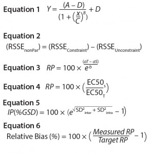
Several characteristics differentiate biological assays from physicochemical methods (12). One key difference is the nonlinear relationship between response and analyte concentration. Binding assay response–function curves result from interactions between analytes and their target antibodies and/or other binding reagents. The response could be directly or indirectly proportional to analyte concentration, depending on whether the assay is competitive or noncompetitive. Such a log(concentration)–response relationship generates nonlinear response of sigmoidal shape. The model commonly used for curve-fitting analysis of sigmoidal symmetric curves is the four-parameter logistic (4-PL) regression model shown as Equation 1. Here, Y is the response, A is the response at zero analyte concentration, D is the response at infinite analyte concentration, C is the inflection point — also known as EC50 ((A + D) ÷ 2) — B is the slope that defines the steepness of the curve, and x is the analyte log(concentration).
A 4-PL function requires a sufficient number of concentrations or dilutions to fit the model. One concentration is commonly used (or two would be better) to support each asymptote (parameters A and D) and at least three (or better, four) concentration points in the linear part of the curve. The linear part of a 4-PL function often is defined as concentrations near the center of the response region. B parameter (slope) should be ∼1, meaning that the concentration points are well distributed spatially.
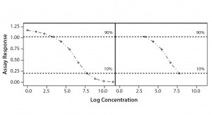
Some biological assays assume that the concentration–response function approximates a straight line over a limited range of concentrations. In this case, a linear regression model can be used to fit the data generated. As stated above, one characteristic of the bioassay is that the log(dose) responses are not linear. A common strategy to overcome that aspect is to identify and select the approximately linear region of the full response curve. This region is often defined as the range between 10% and 90% of a response when a 4-PL model is applied and the data are rescaled to the asymptotes.
The mathematics are straightforward for a linear dose– response function. Parallelism can be determined using parameter comparison methods (e.g., difference of slopes or ratio of slopes). For the parallel-curve model, parallelism assessment should include consideration of the entire full dose– response curve. Two approaches can be found in the literature. We evaluate each dose–response parameter (slope, upper, and lower asymptotes) independently or with a composite measure (e.g., residual-sum-of- squared-errors, RSSE) (13).
Parallel-Line Model: We defined the linear region of dose–response curves as the log concentration points that fell between 10% and 90% of the range between the lower and upper 4-PL asymptote (Figure 1). We set a criterion of having at least four points in the selected linear range to accept the dose–response curve and to proceed with data analysis. In addition, we assessed our linearity assumption by checking linearity of the selected range through the quadratic coefficient of the standard and sample dose–response curves. In case of perfect linearity, the quadratic coefficients should be equal to zero.
We assessed our similarity assumption by checking parallelism through the slope ratios for each couple standard/sample dose-response curve. For perfect parallelism, the slope ratio should be equal to one.
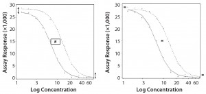
Parallel-Curve Model: In this case study, we used a composite measure to assess similarity. A composite measure considers all parameters (slope, upper and lower asymptotes) together in a single measure called nonparallelism residual sum of squared errors (RSSEnonPar) (13). It is a direct measure of the amount of nonparallelism between two curves, and it ranges from zero (perfect parallelism) to infinity (less and less parallel). RSSEnonPar measures the difference between the residual variability when the parameters of two curves (slope and asymptotes) are constrained to be equal (constraint model) and the residual variability when the parameters (slope and asymptotes) are different for each curve (unconstraint model) (Figure 2), as shown in Equation 2.
Define an Equivalence Interval to Measure Nonsimilarity
Similarity is the key assumption to be fulfilled before calculating relative potency. It implies that standard and test-sample dose–response curves share common functional parameters. When this condition is met, the horizontal shift (along the log concentration axis) between the standard and test sample is the measure of relative potency.
USP strongly recommends implementation of equivalence testing instead of difference tests. An equivalence approach for similarity assesses whether the measure of nonsimilarity is contained within specified equivalence bounds. So it will not allow samples with nonsimilarity measures outside the equivalence boundaries to be declared as similar. An equivalence approach offers the advantage of not penalizing too-precise (“good”) results (producer’s risks) and of rejecting (“bad”) results with decreased replication or precision (consumer’s risk). The big challenge is to define appropriate equivalence limits (acceptance criteria) for similarity measures that will allow accepting good response–function curves and rejecting aberrant ones.
Four different approaches are described in USP chapter <1032> to support the definition of equivalence limits (Figure 3). The first three approaches are based on compiled historical data that compare a standard to itself. The advantage of using historical data is to better control the false-failure rate (the rate of failing a sample that is, in fact, acceptable). The drawback of that method is that it does not allow control of the false-pass rate (the rate of passing a sample that has an unacceptable difference in performance relative to a standard).
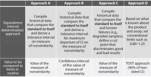
Figure 3: Different approaches presented in USP to help defining equivalence intervals; TOST = two one-sided test, CI = confidence interval
In this case study, we decided to implement the equivalence testing by using approach A (Figure 3). We performed a prevalidation study to establish equivalence intervals for both approaches. We derived those intervals as tolerance intervals for the different measures of nonsimilarity (slope ratio and composite measure).
Determine Whether the Nonsimilarity Value is Within the Equivalence Interval
We assessed parallelism by comparing the nonsimilarity value to the corresponding equivalence interval. Results of the nonsimilarity measure obtained during validation exercise were compared to equivalence intervals determined in the second step.
For parallel-line models, we assessed nonsimilarity (parallelism) using the slope ratio between the standard and test sample dose-responses. Parallelism is accepted when slope ratio for the couple standard/sample is contained inside the equivalence interval. A linear model presupposes linearity of a dose-response. That characteristic also can be assessed using equivalence testing through the quadratic coefficient of each dose–response.
For parallel-curve models, two response function curves (standard/ sample) are considered to be parallel when the RSSEnonPar measure is less than or equal to the equivalence limit.
Relative Potency Calculation
As soon as the similarity assumption is demonstrated, a sample’s relative potency can be calculated. To compute relative potency in a parallel-line model, a linear regression with a common slope and different intercepts is fitted on the linear range selected from the 4-PL curve of the couple standard/sample. Relative potency (RP in %) is computed using Equation 3. Here, aT is the test-sample intercept, aS is the standard-sample intercept, and b is the common slope.
In a parallel-curve model, for each couple standard /test sample, the relative potency (RP %) is computed using Equation 4. Here, EC50S and EC50T are the EC50 parameters of the reference sample and of the test sample, respectively.
Validation
We performed a validation exercise to evaluate the method’s performance (intermediate precision and relative accuracy). A validation should demonstrate that a method is suitable for its intended use, in this case for routine quality control activities. However, because the amount of historical data is limited in the initial stage of drug development, we did not set predetermined method- performance specifications. Instead, we used validation objectives based on commonly accepted acceptance criteria for ligand binding assays (see Intermediate Precision and Relative Accuracy sections below).
To mimic under- and over-potent samples, we diluted reference material at five concentration levels covering the range between 50% and 200% of the nominal concentration. These percentages constitute the target relative potencies in the validation. For these calculations, the RP measurements were log-transformed because the RP are log-distributed.
Two operators performed validation experiments over five days. Each operator analyzed independent preparations of standard (two per plate) and samples in three independent plates per day. Relative potencies were calculated by comparing each sample log(dose)-response curve to the two standard log(dose)-response curves inside each plate.
Intermediate precision (IP) measures the influence of factors that will vary over time after an assay is implemented (e.g., multiple analysts or instruments). We assessed IP by using a variance component analysis taking into account the factor series. Each series was defined as a unique combination of three factors: operator, day, and plate. We combined resulting estimations of variance components of the interseries (SD2inter) and intraseries (SD2intra) variation to establish overall IP of the assay at each level. The value was expressed as percent geometric standard deviation (%GSD) as shown in Equation 5. We set IP at each target RP level ≤20% as the target acceptance criterion.
Relative accuracy is the relationship between measured RPs and target RPs. We assessed accuracy in two steps: through a trend in relative bias across levels and at individual levels.
We measured trend in bias using the estimated slope of linear regression between measured log RP and target log RP. A slope = 1 corresponds to the case in which measured RPs are equal to target RP. An equivalence test determines whether the slope can be considered as equal to 1 (no trend in bias). As an acceptance criterion, the 90% confidence interval of the estimated slope had to be inside the equivalence margin (0.8–1.25). We calculated the relative bias at each level, as shown in Equation 6. We set the confidence interval of the relative bias at each level ≤30% as the target acceptance criterion.
Total-Error Approach
We assessed method bias and variability individually by using the USP <1033> approach. To have a comprehensive measure of method performance, we applied the total-error approach (14) to both models. This statistical approach combines in a single measure the estimates of systematic and random errors, which is the combination of trueness and precision. A total-error profile is obtained by linking the lower bound and upper bound of the β-expectation tolerance limits calculated at each target relative potency level. The profile can be used as a statistical tool for controlling the risk of accepting methods that do not fulfill suitability requirements. If the tolerance interval lies within acceptance limits, there is a chosen probability (e.g., 95%) that at least a proportion β of future measured assay values are inside predefined acceptance limits (A, B; e.g., ±30%). The method is then considered suitable for its intended use. Predefined acceptance limits must be chosen according to the intended use of the method. For this case study, we used a beta version of Seelva 2.0 from Arlenda to calculate the total-error profile.
Results
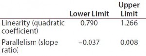
Table 1: Equivalence margins for parallel-line model calculated following USP guidance approach A (derived as a tolerance interval for the measure of nonsimilarity, quadratic coefficient and slope ratio)
Suitability Testing, Parallel-Line Model: Our equivalence intervals for the quadratic coefficient and slope ratio were based on historical data obtained before validation. We defined linear regions from the 4-PL curves of 56 reference samples. We estimated 56 quadratic coefficients and 196 slope ratios from all possible combinations of two dose-response curves inside each plate. We used estimated values to define equivalence intervals for linearity and parallelism (Table 1).
During the validation exercise, we evaluated 276 standard/sample couples for suitability testing using the equivalence intervals shown in Table 1. Of the total 276 standard/sample couples, 181 passed the suitability tests for linearity and parallelism (rejection rate = 34.4%). We evaluated validation parameters on the 181 relative potencies calculated from the samples that passed the suitability tests.

Table 2: Equivalence margin for parallel-curve model was calculated following USP guidance approach A (derived as a tolerance interval for the measure of nonsimilarity, RSSEnonPar). Because the RSSEnonPar ranges from 0 to ∞, only the upper limit is calculated.
Parallel-Curve Model: We calculated the equivalence interval for the composite measure (RSSEnonPar) based on the 196 RSSEnonPar estimated from all possible combinations of two dose– response curves inside each plate obtained from the 4-PL curves of the 56 reference samples. Table 2 lists that interval. During the validation exercise, we evaluated 276 standard/sample couples for suitability testing using the equivalence interval shown in Table 2. Out of that total, 265 standard/sample couples passed the suitability tests for parallelism (rejection rate 4%). The validation parameters thus were evaluated on the 265 relative potencies calculated from the samples that passed the suitability tests.
Intermediate Precision: We used the RPs that passed suitability testing to estimate the IP of both datasets. Table 3 shows the absolute IP by target RP level and the overall IP for both datasets. IP is expressed as percent geometric coefficient of variation (%GCV). For the parallel-line model, IP ranges 12.1–18.7%, according to the level, and maximum IP value is observed for the 71% target level (18.7%).

Table 3: Absolute intermediate precision (by level) and overall intermediate precision for parallel-line and parallel-curve approaches
For the parallel-curve model, IP varies from 12.6% to 15.6% according to the level, and maximum IP value is observed for the 71% target level (15.6%). Results obtained for both approaches are comparable in terms of absolute (by level) and overall IP. Overall IP is <20% for both models. However, a better precision is obtained for the parallel- curve model (13.9% compared with 15.5%).
Accuracy: We used the RPs that passed suitability testing to estimate relative accuracy. We first evaluated relative accuracy using the trend in relative bias across levels. Table 4 shows the slopes obtained from the linear regression and with their 90% confidence intervals (CIs) for both datasets.
Both approaches met the acceptance criterion because the 90% CI of their estimated slopes fell inside the acceptance margin (0.8– 1.25). Because we did observed no trend in relative bias, we computed it at each level. Table 5 lists the relative bias at each individual level with the corresponding 90% CI for both models. The acceptance criterion was met for both approaches because the 90% CI of relative bias at each individual level is ≤30%.
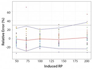
Figure 4: Total-error profile for parallel-line approach; the plain red line represents the relative bias, the dashed lines the β-expectation tolerance limits and the dotted lines the acceptance limits (–30% and +30%). The dots represent the relative error of the relative-potency (RP) values plotted at the corresponding RP level.
Total-Error Approach: Figure 4 shows the total-error profile for the parallel-line approach, and Figure 5 shows it for the parallel-curve approach. The plain red line represents the relative bias, the dashed lines represents the β-expectation tolerance limits, and the dotted lines are the acceptance limits. The dots represent the relative error of RP values plotted at the corresponding RP level.
We set acceptance limits at –30% and +30%, selected according to the intended use of the potency assay, with a risk of having measurements outside acceptance limits of 10%.
The potency assay is considered to be valid in the range for which the total-error profile is within acceptance limits. Further measurements of unknown samples will be included within the tolerance limits with a given probability. When the tolerance interval is within acceptance limits, it means that with a risk of 10% (α = 10%), at least 90% (proportion β) of future results generated by the method will be included within the acceptance criteria.
Based on the total-error profile, we calculated the range of the potency assay as the concentration at which the β-expectation tolerance interval crosses the acceptance limits set at ±30%. For the parallel-line approach, the calculated range is 50.0–169.6%, and for the parallel- curve approach that range is between 50.0% and 188.9%. For both models, analytical ranges obtained with the total-error approach are comparable and do not significantly differ from results obtained when using the USP validation — even if for the total error approach, the ranges are slightly tighter.
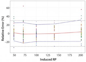
Figure 5: Total-error profile for parallel-curve approach; the plain red line represents the relative bias, the dashed lines the β-expectation tolerance limits and the dotted lines the acceptance limits (–30% and +30%). The dots represent the relative error of the RP values plotted at the corresponding RP level.
Discussion
Considering the results obtained for IP, trend in bias, and relative accuracy, we concluded that the relative potency method was valid for the 50–200% range of nominal concentration for both models (parallel-line and parallel-curve). However, some discrepancies between the two approaches exist. We have determined how to improve the statistical approach presented in this case study.
Rejection Rate: We saw a significant difference in rejection rates. Based on the system suitability criteria defined for each model, 34.4% of dose–response curves (95 out of 276) were discarded in the linear model (similarity assessed based on slope ratios) compared with 4% (11 dose–response curves out of 276) in the parallel-curve approach (similarity assessed based on RSSE values).
One reason for the low rejection rate observed in the parallel-curve approach could be that equivalence limits were too wide. That led to the acceptance of dose–response curves that in reality should have been discarded because of potential nonparallelism. In other words, the equivalence limit set for the parallel-curve approach wouldn’t be strict enough to discriminate between “bad” and “good” dose–response curves, ultimately increasing consumers’ risk. By erroneously accepting curves that do not meet the similarity assumption, meaningless RP values might be taken into consideration, which can influence the evaluation of validation characteristics.
On the other hand, we could apply the same reasoning to the parallel- line approach. In such a case, too tight equivalence margins might have caused the high rejection rate. Therefore, “good” dose–response curves might have been erroneously rejected, increasing producers’ risk.
Nevertheless, comparing validation results between both approaches indicates that the influence of the difference on the rejection rate is quite limited. In fact, even with this difference, we obtained comparable validation results in terms of IP, trend in relative bias, and relative accuracy for the 50–200% range. We confirmed our validation results by applying the total-error approach, the combination of the systematic errors (bias) and random errors (precision) in one single measure (total-error profile). As mentioned above, the total-error profile is a powerful prediction tool that helps us control the risk of accepting an unsuitable assay. In our case study, the analytical range derived from the total-error profile is comparable for both models.
Even if validation results are comparable between both models, the estimation of the validation characteristics is more precise in the parallel-curve model, especially in terms of precision. That could be explained by the higher number of RPs values used for the validation exercise with the parallel-curve model. But the parameters used to compute RP in a linear model can be less accurately estimated, which can lead to a higher residual variability. In fact, the linear range is selected from sigmoidal response curves with consequence on the goodness of fit of the linear model (15). In addition, as described in USP <1032>, a linear model must be used with caution because the apparently linear region may shift over the time with an effect on the parallelism. Such an effect could lead to a higher rejection rate.
Methodology Used to Define Equivalence Limits: As described by Hauck et al., approach A described in USP<1032> — tolerance interval derived from historical values of nonparallelism — is the simpler approach to determine equivalence limits, and it does not take into consideration the imprecision of nonsimilarity replicates (8). As the authors present, that point could be addressed by considering the confidence intervals of the nonsimilarity measure, which corresponds to approach B in USP <1032>. In that approach, equivalence limits are set as a nonparametric tolerance interval derived from the maximum departure of the confidence interval of nonsimilarity measure.
We defined equivalence limits based on approach B on the linear model data (data not shown). The rejection rate dropped down to 11.2%, which supports the hypothesis that equivalence limits set with the approach A were too strict. Because of statistical constrains, we are not yet able to apply approach B to the nonsimilarity RSSE values. Therefore, no comparison of the equivalence limits calculated by using approach B on both models was performed.
USP<1032> presents a third approach (approach C). Equivalence limits are defined based on historical data from reference material and known failures (e.g., degraded samples). This approach allows defining a cut point to discriminate between good and bad results. However, the methodology’s limitation lies on the degree of sample degradation, which can directly influence the cut point.
Again, the precision of the equivalence limits definition will depend on the amount of historical data. In the early phases of drug development, such limits can be considered as provisional and should be refined throughout drug development using data collected over time.
Perspectives
Considering the validation characteristics and rejection rates between both tested methodologies (linear and nonlinear), the preferred approach for relative potency determination in this case study is the parallel-curve model. Using it, we obtained a lower rejection rate without influencing method performance.
Relative potency is a measure of how much a test preparation is diluted or concentrated relative to a standard (1, 4). Although a linear model is considered to be the easiest model to demonstrate parallelism (8, 9), the risk of having the linear part drift over time — altering parallelism — is high. In addition, sample degradations usually affect the dose– response at asymptote levels before affecting slope, which is the only parameter evaluated in the parallel- line model. Therefore, by considering only the linear part, scientists might fail to identify low levels of product degradation because of a lack of information of upper asymptotes. When full dose–response curves are used to test similarity, both asymptotes can be taken into consideration to compare a standard and sample. However, that approach implies a bigger statistical effort to determine the degree of parallelism between both functions and to verify similarity assumption.
When two response curves are not parallel, the distance between their concentration points is not constant, so the smallest variation can affect parallelism. This underlines the importance of using the correct measure of nonsimilarity to assess parallelism (the condition required before calculating a relative potency).
For our case study, we used a composite measure (RSSEnonPar) that considers all parameters together in a single measure, as proposed by the USP guidance. The composite measure is not an absolute measure. Therefore, it can’t be compared across methods and is highly influenced by the readout (absorbance, relative fluorescence and luminescence values). USP also proposes assessing parallelism based on fitting model parameters. That can be achieved through an intersection-union test (IUT), which jointly assesses the equivalence of slope and lower and upper asymptotes (16, 17). In the IUT method proposed by Jonkman for each of these three parameters, a ratio between the obtained values for the test and the reference parameters is calculated, together with its confidence interval. Yang et al. propose a modified IUT based on three measures derived or directly obtained from the parameters of the curves:
- The effective window (the difference between lower and upper asymptotes)
- The slope of the dose–response curve at EC50 (the difference between upper and lower asymptotes multiplied by the hill slope divided by four),
- The upper asymptote.
For each measure, a ratio between the obtained values for the test and the reference curve is calculated, together with its confidence interval. Parallelism of the test and reference curves is accepted only if the confidence interval of each of the three ratios is fully within a ratio-specific equivalence margin previously defined.
Using RSSEnonPar metrics is a simple, quick, and complete method to test parallelism of 4-PL curves. But it would be interesting, in a future exercise, to compare both approaches (RSSEnonPar and IUT).
References
1 USP Chapter <1032> Design and Development of Biological Assays. USP Pharmacopeial Convention: Rockville, MD, 2013.
2 Robinson CJ, et al. Assay Acceptance Criteria for Multiwell-Plate-Based Biological Potency Assays. BioProcess Int. 12(1), 2014: 30–41.
3 Rieder N, et al. The Roles of Bioactivity Assays in Lot Release and Stability Testing. BioProcess Int. 8(6) 2010: 33–42.
4 Singer R, Lansky DM, Hauck WW. Bioassay Glossary. Stimuli to the Revision Process. Pharmacopeial Forum 32, 2006: 1359–1365.
5 USP Chapter <111> Design and Analysis of Biological Assays. US Pharmacopeial Convention: Rockville, MD, 2014.
6 USP Chapter <1033> Biological Assay Validation. USP Pharmacopeial Convention: Rockville, MD, 2013.
7 USP Chapter <1034> Analysis of Biological Assays. US Pharmacopeial Convention: Rockville, MD, 2013.
8 Hauck WW, et al. Assessing Parallelism Prior to Determining Relative Potency. PDA J. Pharma. Sci. Technol. 59(2), 2005: 127–137.
9 Callahan JD, Sajjadi NC. Testing the Null Hypothesis for a Specified Difference: The Right Way to Test for Parallelism. BioProcessing J. 2(2), 2003: 71–77.
10 Burdick RK, et al. Statistical Methods for Validation of Procedure Accuracy and Precision: Stimuli to the Revision Process. Pharmacopeial Forum 39(3) 2013.
11 Chapter <1210> Statistical Tools for Method Validation. Pharmacopeial Forum 40(5) 2014.
12 Findlay JWA, et al. Validation of Immunoassays for Bioanalysis: A Pharmaceutical Industry Perspective. J. Pharm. Biomed. Analysis 21, 2000: 1249– 1273.
13 Gottschalk PG, Dunn JR. Measuring Parallelism, Linearity, and Relative Potency in Bioassay and Immunoassay Data. J. Biopharm. Stat. 15(3) 2005: 437–463.
14 Hoffman D, Kringle R. A Total- Error Approach for the Validation of Quantitative Analytical Methods. Pharma. Res. 24(6) 2007: 1157–1164.
15 Findlay JWA, Dillard RF. Appropriate Calibration Curve Fitting in Ligand Binding Assay. AAPS J. 9(2) 2007: 260–267.
16 Jonkman JF, Sidik K. Equivalence Testing for Parallelism in the Four- Parameter Logistic Model. J. Biopharm. Stat. 19, 2009: 818–837.
17 Yang H, et al. Implementation of Parallelism Testing for Four Logistic Model in Bioassays. PDA J. Pharm. Sci. Technol. 66, 2012: 262–269.
Corresponding author Erica Bortolotto, PhD, is a scientist of bioassay development in Analytical Sciences for Biologicals at UCB Pharma SA, Chemin du Foriest, B-1420 Braine l’Alleud, Belgium, 32 2 386 57 40; www.ucb.com; erica.Bortolotto@ucb.com. Rejane Rousseau is a statistician at Arlenda SA in Liege, Belgium; Bianca Teodorescu is an associate director of nonclinical statistics at UCB Biopharma SPRL; Annemie Wielant is a scientist in bioassay development at UCB Pharma SA; and Gael Debauve is an associate director of bioassay development at UCB Pharma SA.


